Author: Alexey Dosovitskiy, Lucas Beyer, Alexander Kolesnikov, Dirk Weissenborn, Xiaohua Zhai, Thomas Unterthiner, Mostafa Dehghani, Matthias Minderer, Georg Heigold, Sylvain Gelly, Jakob Uszkoreit, Neil Houlsby
Date: October 22, 2020 (Last revised: June 3, 2021)
Link: https://arxiv.org/abs/2010.11929
An Image is Worth 16x16 Words: Transformers for Image Recognition at Scale
Introduction
The Vision Transformer (ViT) revolutionized computer vision by demonstrating that pure transformer architectures—without any convolutional components—can achieve state-of-the-art performance on image classification tasks. This breakthrough challenged the long-held assumption that convolutional neural networks (CNNs) are essential for computer vision.
The CNN Dominance Era
Before ViT, computer vision was dominated by convolutional neural networks:
- CNNs: Designed specifically for image data with inductive biases
- Attention in vision: Limited to augmenting CNNs or replacing specific components
- Architectural assumption: Convolutions were considered necessary for visual tasks
The Transformer architecture, despite revolutionizing NLP, had limited success in pure vision applications.
ViT's Revolutionary Insight
The key insight: CNNs are not necessary for excellent image recognition performance.
Instead of adapting Transformers to work with CNNs, ViT applies a pure Transformer directly to sequences of image patches, treating images similarly to how NLP models treat text sequences.
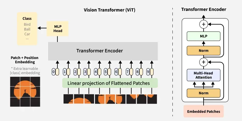
Architecture Overview
Image Patch Embedding
The core innovation is treating an image as a sequence of patches:
class PatchEmbedding(nn.Module):
    def __init__(self, image_size=224, patch_size=16, in_channels=3, embed_dim=768):
        """
        Convert image to sequence of patch embeddings

        Args:
            image_size: Input image size (assumes square images)
            patch_size: Size of each patch (16x16 pixels)
            in_channels: Number of input channels (3 for RGB)
            embed_dim: Embedding dimension
        """
        super().__init__()
        self.image_size = image_size
        self.patch_size = patch_size
        self.num_patches = (image_size // patch_size) ** 2

        # Linear projection of flattened patches
        self.projection = nn.Conv2d(
            in_channels,
            embed_dim,
            kernel_size=patch_size,
            stride=patch_size
        )

    def forward(self, x):
        # x shape: (batch_size, channels, height, width)
        # Output shape: (batch_size, num_patches, embed_dim)

        x = self.projection(x)  # (B, embed_dim, H/P, W/P)
        x = x.flatten(2)  # (B, embed_dim, num_patches)
        x = x.transpose(1, 2)  # (B, num_patches, embed_dim)

        return x
The "16x16 Words" Concept
For a 224×224 image with 16×16 patches:
Image: 224 × 224 pixels
Patch size: 16 × 16 pixels
Number of patches: (224/16) × (224/16) = 14 × 14 = 196 patches

Each patch becomes a "word" in the sequence!
This is the origin of the title: "An Image is Worth 16×16 Words"
Complete ViT Architecture
class VisionTransformer(nn.Module):
    def __init__(
        self,
        image_size=224,
        patch_size=16,
        num_classes=1000,
        embed_dim=768,
        depth=12,
        num_heads=12,
        mlp_ratio=4.0
    ):
        super().__init__()

        # Patch embedding
        self.patch_embed = PatchEmbedding(
            image_size, patch_size, 3, embed_dim
        )
        num_patches = self.patch_embed.num_patches

        # CLS token (for classification)
        self.cls_token = nn.Parameter(torch.zeros(1, 1, embed_dim))

        # Positional embeddings
        self.pos_embed = nn.Parameter(
            torch.zeros(1, num_patches + 1, embed_dim)
        )

        # Transformer encoder blocks
        self.blocks = nn.ModuleList([
            TransformerBlock(embed_dim, num_heads, mlp_ratio)
            for _ in range(depth)
        ])

        # Classification head
        self.norm = nn.LayerNorm(embed_dim)
        self.head = nn.Linear(embed_dim, num_classes)

    def forward(self, x):
        B = x.shape[0]

        # Patch embedding
        x = self.patch_embed(x)  # (B, num_patches, embed_dim)

        # Add CLS token
        cls_tokens = self.cls_token.expand(B, -1, -1)
        x = torch.cat((cls_tokens, x), dim=1)  # (B, num_patches+1, embed_dim)

        # Add positional embedding
        x = x + self.pos_embed

        # Transformer blocks
        for block in self.blocks:
            x = block(x)

        # Classification
        x = self.norm(x)
        cls_output = x[:, 0]  # Extract CLS token
        logits = self.head(cls_output)

        return logits
Transformer Block
Each transformer block contains standard components:
class TransformerBlock(nn.Module):
    def __init__(self, embed_dim, num_heads, mlp_ratio=4.0):
        super().__init__()

        # Multi-head self-attention
        self.attention = MultiHeadAttention(embed_dim, num_heads)
        self.norm1 = nn.LayerNorm(embed_dim)

        # Feed-forward network
        mlp_hidden_dim = int(embed_dim * mlp_ratio)
        self.mlp = MLP(embed_dim, mlp_hidden_dim)
        self.norm2 = nn.LayerNorm(embed_dim)

    def forward(self, x):
        # Attention with residual connection
        x = x + self.attention(self.norm1(x))

        # MLP with residual connection
        x = x + self.mlp(self.norm2(x))

        return x
Model Variants
ViT comes in multiple sizes:
ViT-Base
- Layers: 12
- Hidden size: 768
- MLP size: 3072
- Heads: 12
- Parameters: 86M
ViT-Large
- Layers: 24
- Hidden size: 1024
- MLP size: 4096
- Heads: 16
- Parameters: 307M
ViT-Huge
- Layers: 32
- Hidden size: 1280
- MLP size: 5120
- Heads: 16
- Parameters: 632M
Training Strategy
Pre-training on Large Datasets
ViT's success relies heavily on pre-training with large datasets:
# Pre-training datasets
JFT-300M: 300 million images (Google internal)
ImageNet-21k: 14 million images, 21k classes
ImageNet-1k: 1.3 million images, 1k classes

# Training procedure
1. Pre-train on large dataset (JFT-300M or ImageNet-21k)
2. Fine-tune on downstream tasks
3. Achieve state-of-the-art results
The Data Scale Effect
A key finding: ViT requires more data than CNNs to reach optimal performance
Small datasets (ImageNet-1k only):
- CNNs: Excellent performance
- ViT: Underperforms CNNs

Large datasets (ImageNet-21k, JFT-300M):
- ViT: Matches or exceeds CNN performance
- Scales better with data
This is because:
- CNNs have built-in inductive biases for images (locality, translation equivariance)
- ViT learns these patterns from data
- With sufficient data, ViT learns better representations
Experimental Results
ImageNet Classification
When pre-trained on JFT-300M and fine-tuned on ImageNet:
| Model | Accuracy | Pre-training Cost |
|---|---|---|
| BiT-L (ResNet) | 87.5% | High |
| Noisy Student | 88.4% | Very High |
| ViT-H/14 | 88.6% | Lower |
Transfer Learning Performance
ViT excels at transfer learning across multiple benchmarks:
Few-shot learning:
- Competitive or better than CNNs
- Scales efficiently with pre-training data
VTAB (Visual Task Adaptation Benchmark):
- Strong performance across diverse tasks
- Better generalization than CNN counterparts
Computational Efficiency
Training Efficiency
# Comparison for similar performance

ResNet-152 (BigTransfer):
- Parameters: ~60M
- Pre-training: 9k TPUv3 core-days

ViT-L/16:
- Parameters: 307M
- Pre-training: 2.5k TPUv3 core-days
- Result: Better accuracy with ~4x less computation!
Inference Efficiency
ViT offers excellent inference throughput:
Patches processed in parallel (unlike CNN's sequential convolutions)
Self-attention allows global context at every layer
Efficient on modern hardware (GPUs/TPUs)
Attention Visualizations
One of ViT's advantages is interpretability through attention maps:
def visualize_attention(model, image, layer_idx=11):
    """
    Visualize attention patterns in ViT

    Args:
        model: Trained ViT model
        image: Input image
        layer_idx: Which transformer layer to visualize
    """
    # Get attention weights from specified layer
    with torch.no_grad():
        attentions = model.get_attention_maps(image)
        attention = attentions[layer_idx]

    # Average over heads
    attention = attention.mean(dim=1)

    # Attention from CLS token to patches
    cls_attention = attention[0, 0, 1:]

    # Reshape to image grid
    num_patches = int(cls_attention.shape[0] ** 0.5)
    attention_map = cls_attention.reshape(num_patches, num_patches)

    # Visualize
    plot_attention_map(attention_map, image)
Key observations from attention patterns:
- Early layers: Local, texture-focused attention
- Middle layers: Object parts and structure
- Late layers: Semantic, whole-object attention
Hybrid Architectures
The paper also explored ViT-hybrid models:
class HybridVisionTransformer(nn.Module):
    def __init__(self, cnn_backbone, transformer_config):
        super().__init__()

        # CNN feature extractor (e.g., ResNet50)
        self.cnn_backbone = cnn_backbone

        # Use CNN features as "patches"
        self.transformer = VisionTransformer(
            patch_size=1,  # Already extracted features
            **transformer_config
        )

    def forward(self, x):
        # Extract CNN features
        features = self.cnn_backbone(x)

        # Process with transformer
        output = self.transformer(features)

        return output
Findings:
- Hybrids perform slightly better at smaller scales
- Pure ViT outperforms hybrids at larger scales
- Demonstrates that CNNs are not necessary
Position Embeddings
ViT uses learnable position embeddings:
# 1D position embeddings
self.pos_embed = nn.Parameter(
    torch.zeros(1, num_patches + 1, embed_dim)
)

# During training, the model learns spatial relationships
# Despite being 1D, it learns 2D spatial structure!
Experiments showed:
- 1D embeddings work as well as 2D
- Model learns spatial relationships from data
- Pre-training learns transferable position patterns
Impact on Computer Vision
ViT's impact has been transformative:
1. Architectural Paradigm Shift
Demonstrated that domain-specific architectures (CNNs) are not always necessary:
- Enabled architecture unification across domains
- Paved the way for multi-modal models
2. Scaling Laws
Showed that vision models scale similarly to NLP models:
- Performance improves with model size
- Performance improves with data size
- Follows predictable scaling laws
3. Research Directions
Inspired numerous follow-up works:
- DeiT: Data-efficient image transformers
- Swin Transformer: Hierarchical vision transformers
- BEiT: BERT pre-training for images
- MAE: Masked autoencoders for vision
- CLIP: Contrastive language-image pre-training
4. Industry Adoption
Widely adopted in production systems:
- Image classification
- Object detection (DETR, ViT-based detectors)
- Semantic segmentation
- Multi-modal understanding
Best Practices
When to Use ViT
# Good fit:
- Large-scale datasets available
- Pre-trained models for transfer learning
- Need for interpretability (attention maps)
- Multi-modal applications

# Consider alternatives (CNNs):
- Small datasets without pre-training
- Extremely resource-constrained environments
- Real-time applications requiring minimal latency
Fine-tuning ViT
# Load pre-trained model
model = VisionTransformer.from_pretrained('vit_large_patch16_224')

# Adjust classification head
model.head = nn.Linear(model.embed_dim, num_classes)

# Fine-tune with higher resolution (optional)
model = model.resize_positional_embedding(384)  # 224 -> 384

# Training
optimizer = AdamW(model.parameters(), lr=1e-4, weight_decay=0.05)
# Use cosine learning rate schedule
# Train for 20-100 epochs depending on dataset size
Limitations and Considerations
1. Data Requirements
- Requires large pre-training datasets
- May underperform CNNs on small datasets
- Pre-training is computationally expensive
2. Fixed Resolution
- Position embeddings are resolution-specific
- Requires interpolation for different resolutions
3. Quadratic Complexity
- Self-attention is O(n²) in sequence length
- Can be limiting for very high-resolution images
Future Directions
ViT opened several research avenues:
Efficient Transformers
Reducing computational complexity:
- Sparse attention patterns
- Linear attention mechanisms
- Hierarchical structures
Self-Supervised Learning
Better pre-training objectives:
- Masked image modeling
- Contrastive learning
- Multi-modal pre-training
Architecture Improvements
Enhancing the basic design:
- Adaptive patch sizes
- Dynamic depth/width
- Hybrid approaches
Conclusion
Vision Transformer represents a landmark achievement in computer vision. By demonstrating that pure transformer architectures can match or exceed CNN performance on image recognition tasks, ViT fundamentally challenged assumptions about what architectures are necessary for visual understanding.
Key Contributions:
- Architectural simplicity: Pure transformer, no convolutions needed
- Scalability: Excellent performance scaling with data and model size
- Efficiency: Superior computational efficiency compared to CNNs at scale
- Transferability: Strong transfer learning across diverse visual tasks
- Interpretability: Attention maps provide insights into model behavior
The impact of ViT extends beyond image classification, influencing object detection, segmentation, video understanding, and multi-modal learning. It established transformers as a universal architecture capable of handling diverse data modalities, paving the way for foundation models that can process text, images, audio, and more within a unified framework.
As the field continues to evolve, ViT's principles remain foundational to modern computer vision, and its legacy continues through countless derivative works and applications in both research and industry.
Citation:
@article{dosovitskiy2020image,
  title={An Image is Worth 16x16 Words: Transformers for Image Recognition at Scale},
  author={Dosovitskiy, Alexey and Beyer, Lucas and Kolesnikov, Alexander and Weissenborn, Dirk and Zhai, Xiaohua and Unterthiner, Thomas and Dehghani, Mostafa and Minderer, Matthias and Heigold, Georg and Gelly, Sylvain and others},
  journal={arXiv preprint arXiv:2010.11929},
  year={2020}
}